FastAI Deep Learning Journey Part 9: Building Simple Recommender Systems using collaborative filtering with fastAI

The following post is a modest yet solid start to the topic of recommender systems. In the following notebook collaborative filtering repo, we show how to recommend movies that users are likely to like.

What I find very interesting of the method used, in our case collaborative filtering, is that we do not need to know any metadata from the consumer and the items/products, only a metric of interaction with users and items (such as ratings, clicks, purchase, visualization). That goes at the price of data sparsity (many items without sufficient interactions), cold start problem (how to make recommendations on totally new users or items) and representation bias (we do not have a balanced sample of items/users interactions).

At the end of the post I will make some suggestion for how to overcome those issues. Let's start explaining collaborating filtering in a nutsell.

Collaborative filtering

Taking our film example will be of use here. Imagine that I am keen to watch sci-fi space related films, but specially the classic ones, as the new ones are too action heavy. We can define the level of scifi and newness as the two latent factors driving my (and many sci-fi classic viewers like me) viewing experience. Let's assume we have two possible movies, one is the very first movie of Start Wars, and the second is the last movie of Star Trek. We can represent my user latent factors and the two movies as follows:

Alan's latent factors : [ 1, 1] first item correspont to very high fiction, and the second to classic
Star Wars a New Hope (1970's movie0 : [1,1] is scifi and a classic
Star Trek First Frontier (2020) : [1,-1] is sci-fi but very new and action heavy

We can predict my utility of each films by simply multiplying each latent factor from me (the user) to each movie, or do the dot_product, and get 1*1 +1*1 = 2 for Start Wars Episode IV and 1*1+1*-1=0 for Star Trek First Frontier. That shows that Star Wars is a better match as it is both classic and sci-fi. This example is trivial, but we will be able to do that not only for users like me, but for many other movies, users and potentially houndreds of latent factors. Our learning goal is to identify which underlying features, revealed by users and item interactions, explain which people will like which movies more or less.

This simply approach is still at the core of many product recommenders. Bare in mind though that production applications require normally additional data for the new items (product metadata) and users (preliminary user genes). For this post we will mainly focused on heavily watched movies and users that have seen plenty of them, so sparsity is less of an issue. The movie lens data used in the course, have filtered out movies that are barely seen or users that have seen many few movies.

How the data would look like normally on collaborative filtering problems

One of the strentghs of the method for me is also in the simplicity of the data required to build a powerful recommendations. We mainly need:

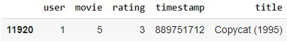
user id
item id - in our example is movie id
interaction score - for movie lens data set is rating (other kpi's could be used for other applications such as purchase, view..)

We can use timestamps, user and product metadata too, but for this very first application we will only use these three columns.

To know more of the data set we will be working on in this post, please check out here: MovieLens.

How are we learning the latent factors

It is still tricky to grasp how can we effectively learn the latent factors, but it is actually quite simple and can be expressed in three steps:

We define a priori the number of latent factors (there are ways to automatically choose them), from now is a predefine number over which we randomize the weights
We make predictions for each user-item /user-movie by applying the dot product of each user latent factor to each movie latent factor. Note that there will be a one to one correspondence between the factors in meaning, but not in values.
We define our loss function, in our case as we are predicting a numeric rating, the loss function could be the MSE (mean squared error)

That's all we need to learn our latent factor values using gradient descent, and as usual, we will need to define the number of epochs, batch size and the like, plus some specific tricks to make the model work well.

Why do we need embeddings to learn the latent factors, and what are embeddings?

In order to learn the latent factors, we will need, for each user and item combination, to look and the index of the item in the item latent factor matrix and do the same for the user. This look up operation is problematic for deep learning as frameworks such as pytorch and tensorflow are efficent for matrix multiplications, not for look ups. One workaround for this is transform our indexes into one-hot encoded vectors and use them for our operation. The problem with that is that is will create a lot of null values and will be slow, but there is a more clever way to do it, which is called the embedding:

"it indexes into a vector using an integer, but has its derivative calculated in such a way that it is identical to what it would have been if it had done a matrix multiplication with a one-hot-encoded vector. This is called an embedding."

This is what an embedding is, and why it is used. Althought I am creating embeddings and using them regularly, I never saw them as a look up trick.

Creating a collaborative filtering model from scratch

In the following, we will create our own model using object oriented programming and the pytorch Module parent class to see how it works:

class CollFilter(Module):
    def __init__(self, n_users, n_movies, n_factors, y_range=(0,5.5)):
        self.user_factors = Embedding(n_users, n_factors)
        self.user_bias = Embedding(n_users, 1)
        self.movie_factors = Embedding(n_movies, n_factors)
        self.movie_bias = Embedding(n_movies, 1)
        self.y_range = y_range
        
    def forward(self, x):
        users = self.user_factors(x[:,0])
        movies = self.movie_factors(x[:,1])
        res = (users * movies).sum(dim=1, keepdim=True)
        res += self.user_bias(x[:,0]) + self.movie_bias(x[:,1])
        return sigmoid_range(res, *self.y_range)

Our CollFilter class contains at the moment two objects:

_init_: requires the number of users, items, factors, and the expected range of the y variable (In our case from 0 to 5.5, which works better than 1 to 5 which is the actual range).

Note that we add user and item/movie bias, the reason for that is that we want to capture:

people who tend to be hard reviewers / very generous reviewers
items/movies that are inherently good or bad, independently of the latent factors, like a quality bias

forward: is going to use to create the predictions, which is an essential input to calculate our loss and grandient descent. Note that we calculate the dotproduct of user and movie factors first and sum the result, and we last add the user and movie bias to the final item/movie predicted score. We use sigmoid range to squeeze our predictions within our expected 0 to 5.5 range.

In order to train our model we simply have to specify for our CollFilter the number of users, movies and latent factors (in our case 5). We create a learner object, that requires our data loader, the model and the loss function. With that in place we can start to train our model for 5 epochs with 0.005 learning rate.

model = CollFilter(n_users, n_movies, 50)
learn = Learner(dls, model, loss_func=MSELossFlat())
learn.fit_one_cycle(5, 5e-3)

This give already a fairly good model, but we can see there is a little overfit, as the validation set top improving significantly while the training loss keep going down. We will show next how to use weight decay to avoid overfitting and improve the performance of the model.

Weight decay, another type of regularization

Weight decay simply adds to our loss the square sum of our parameters, so it penalize large weights, which may slow down training but it will give better generalization.

We can add the concept to our loss function as follows:

loss_with_wd = loss + wd * (parameters**2).sum()

Or the derivative with respect the parameters including weight decay

parameters.grad += wd * 2 * parameters

We can add a custom loss to our learner or simply add the weight decay parameter to our fit call:

model = DotProductBias(n_users, n_movies, 50)
learn = Learner(dls, model, loss_func=MSELossFlat())
learn.fit_one_cycle(5, 5e-3, wd=0.1)

This has not only reduce overfitting but also improve the model performance 7pp. We will look next on how can we used what the model has learned.

What can we learn from the trained embeddings?

As we will see now, it is quite remarkable what can we learn from that data:

Which items are outperforming their scores given their latent factors: the bias term of the items/movies tell us which items are performing well above their expectation given their latent features. That means that if we recommend those movies to people who typically do not see those movies, they are likely to be happy with the content recommended.

movie_bias = learn.model.movie_bias.squeeze()

idxs = movie_bias.argsort(descending=True)[:15]

[dls.classes['title'][i] for i in idxs]

["Schindler's List (1993)", 'Close Shave, A (1995)', 'Wrong Trousers, The (1993)', 'Shawshank Redemption, The (1994)', 'L.A. Confidential (1997)']

2.We can do the same for very bad performers.That could be good to drop from the catalogue, as it adds complexity but no user type will like them.

dxs = movie_bias.argsort()[:5]

      [dls.classes['title'][i] for i in idxs]

['Children of the Corn: The Gathering (1996)',
'Lawnmower Man 2: Beyond Cyberspace (1996)',
'Mortal Kombat: Annihilation (1997)',
'Robocop 3 (1993)',
'Amityville 3-D (1983)']

3. We can infer the meaning of the latent factors (to some extent and depending on the data set and number of latent factors). We can plot directly some items and see the main principal components when we train for many latent factors, or directly with the latent factors when we use something like 3-5. In the below example we can identify award winning films, the level of action and mainstream or pop culture films.

    g = ratings.groupby('title')['rating'].count()
    top_movies = g.sort_values(ascending=False).index.values[:1000]
    top_idxs = tensor([learn.dls.classes['title'].o2i[m] for m in top_movies])
    movie_w = learn.model.movie_factors[top_idxs].cpu().detach()
    movie_pca = movie_w.pca(3)
    fac0,fac1,fac2 = movie_pca.t()
    idxs = list(range(50))
    X = fac0[idxs]
    Y = fac2[idxs]
    plt.figure(figsize=(25,25))
    plt.scatter(X, Y)
    for i, x, y in zip(top_movies[idxs], X, Y):
        plt.text(x,y,i, color=np.random.rand(3)*0.7, fontsize=10)
    plt.show()

4. We can find similar items: we can compute the distance between the item embeddings and find the most similar. If the goal is to recommend something similar, we can find films with very similar item latent factor values computing the cosine similarity.

movie_factors = learn.model.i_weight.weight

idx = dls.classes['title'].o2i['English Patient, The (1996)']

distances = nn.CosineSimilarity(dim=1)(movie_factors, movie_factors[idx][None])

idx = distances.argsort(descending=True)[1]

dls.classes['title'][idx]

Queen Margot (Reine Margot, La) (1994)

5. We can find similar users: we can compute the distance between user embeddings and find the most similar. We can find similar users and recommend movies they liked in the past.

user_factors = learn.model.u_weight.weight + learn.model.u_bias.weight
idx = dls.classes['user'][2]
distances = nn.CosineSimilarity(dim=1)(user_factors , user_factors[idx])
idx2 = distances.argsort(descending=True)[1]
dls.classes['user'][idx2]

313

# we can analyze the ratings and see that they are quite similar of same films

adf = ratings[ratings['user'] == 2]

bdf = ratings[ratings['user'] == 313]

df = adf.merge(bdf[['title', 'rating']], on = 'title', how = 'inner')

df

6. We can predict the rating of unseen movies per user, and use that as item recommendation. That probably nicely become a simple yet powerful application. For any user, we can recommend the film we believe he/she will like the most, after checking the user has not seen it before.

# next I will predict the rating for user 1 on a random film, say 5
movie_factors = learn.model.i_weight.weight + learn.model.i_bias.weight
user_factors = learn.model.u_weight.weight + learn.model.u_bias.weight

def predict(user_factor,movie_factor):
        res = (user_factor*movie_factor).sum()
        return sigmoid_range(res, 0,5.5)

predict(user_factors[1],movie_factors[5])

tensor(3.2241, grad_fn=<AddBackward0>)

# in this case the movie was watched by the user, which we accurately predict
ratings[(ratings['user'] == 1) & (ratings['movie'] == 5)]

# let find the most likely unseen film for the same user
score = []
for n in range(0,len(dls.classes['title'])):
   score.append(predict( movie_factors[n],user_factors[1]))

dls.classes['title'][score.index(max(score))]

'Casablanca (1942)'

Will deep learning help? A more generic approach for collaborative filtering.

Our model is constrained to only using user and item latent factors of the same size, and do not allow us to easily add other variables. The dot product may be also a very simple computation procedure to predict the ratings, and adding non linearities may help, so deep learning can be handy.

In order to do that we will concatenate the user and movie embeddings, and because we will not do the dot product to get the ratings, rather something non-linear and deeper, those embeddings do not need to be of the same size. This will be handy in case we want to build a recommender system that not only use user and item latent factors as input, but any other non latent features (user genes, product features...).

We can use the function get_emb_sz(dls) to get a heuristic based recommendation of the size of the embeddings, which is the minimum between 600 and the round(1.6 * n_cat**0.56).

We can directly use the collab_learner from fastai to apply deep learning, we just need to specify the parameter use_nn = True and the size of each layer, for example [100,50] , will create two hidden layers with 100 and 50 activations respectively.

learn = collab_learner(dls, use_nn=True, y_range=(0, 5.5), layers=[100,50])
learn.fit_one_cycle(5, 5e-3, wd=0.1)

In our case, this is not going to improve the performance achieved with the dotproduct model, but it is more flexible as it allows us to concatenate many more features than the user and item latent factors. This is very important if we want to use deep learning for tabular data, and as we will see in the next post, the only thing that will change is the concatenation of variables.

Pros and Cons of Collaborative Filtering, and further reading

Collaborative filtering requires only data with user id, item id, and a interaction metric we care, to extract very valuable information such as:

Llatent factors that describe each user and item
Similarity between users and items
Detection of highly successful/unsuccessful items, given the latent factors they have (uniquely right or wrong index)
Interpreatable factors that are explanatory of user behaviour (review, purchase...)
Predictions of the expected behaviour of a user on an item (rating, purchase, interaction..)
Accurate recommendations of items unseen or not purchase by the user, with high expected satisfaction

This is wonderful, but we need to recognize the challenges and caviats:

We need a signficant history of users and item interaction
It is hard to get good results for items and users with very little interactions
We cannot use it directly for users or items without history - cold start problem
Our approach did not include timing, novelty, context...

There are some ideas to overcome such pitfalls:

When having short history of items and users, we can narrow down the offering after a questionnaire to get help from the user
For new users or products, we can use some user/item metadata that we know will be good to predict the actual latent factors
We can balance the sample of users and items to avoid overrepresenation of certain users or missing latent factor detection for niche items
We can use a hybrid system based on internal item/user metadata and quickly adjust the recommendations based on the user recent behaviour.

Recommender systems are an incredible rich and complex topic, I recommend to read more or even take dedicated training on the topic. In any case, hope this post is a good stop with fast pytorch and fastAI implementation. Keep on learning by looking at those links!

Concluding remarks

In a world with infinite catalogues, options and very limited time, recommender systems are a way to improve user experience and business performance of any company.

In this post we showed a simple application on movie recommenders using Pytorch and Fastai using collaborative filtering. The beauty of the case study is that we do not need millions of records, nor houndreds of metadata to provide good recommendations to frequent users and movies.

It is important for real life applications to include solutions for the cold start problem, for both users and items. In order to do that, we will need metadata for the user and the item in order to predict reliable the latent factors from those new users and products.

The field is vast, and most business use a hybrid of user and content based recommender framework, which sophistication well exceed the knowledge and time of this blogger.

Last but not least, we showed how to build and user the collaborative learner from fastai and set the ground for a more generic case, which is deep learning for many more data than the latent factors, or in simple works, deep learning for tabular data, we will jump into that in the next post.

For the code backing up this post please go here: CollaborativeFiltering with FastAI REPO!

Alan Fortuny Sicart

Search This Blog