
In the following post, I summarize the key ideas from the fastAI course while doing a deep dives into Convolutions (in 14.1) and Resnets (in 14.2). To complement the content when needed I use the Deep Learning Book from Ian Goodfellow et al. Let's get started!
Kernels and Convolutions
In computer vision problems, before the usage of deep learning, one had to encode almost explicitely which features one want the computer to learn, such as verticat edges. For that purpose, a key operation was the convolution, where a kernel (a matrix aimed to search for an edge for example) was multiplied to the original pixel values in order to create the so called feature map.

As one can see from the image, the kernel is detecting where significant chages on the pixel values happened to detect the edges.
Padding and outputs of convolutions
One thing to note is that the output size after applying the kernel will change to a smaller size, and how much that happens, depends on the kernel size, the stride (length of the step made by the kernel over the pixels) and the amount of padding (how many pixels we add to avoid missing the pixels of the edges of the image).
To calculate the resulting output one can use the following formula:
(n + 2*pad - ks)//stride + 1
Learning the values of the kernels
Ideally, we would like the model to learn the kernel values that are useful for our task. For particularly networks with multiple layers, the actual creation of those kernels manually becomes impossible.
In order to do so we need to ensure the following:
- Enough stride and convolutions that end up with an output of :bs x classes
- Not reducing the activation map too fast, and thefore increase the number of features so we do not decrease the complexity too fast
This is how the code for that will look like:
def conv(ni, nf, ks=3, act=True):
res = nn.Conv2d(ni, nf, stride=2, kernel_size=ks, padding=ks//2)
if act: res = nn.Sequential(res, nn.ReLU())
return res
simple_cnn = sequential(
conv(1 ,4), #14x14
conv(4 ,8), #7x7
conv(8 ,16), #4x4
conv(16,32), #2x2
conv(32,2, act=False), #1x1
Flatten(),
)
The following architecture ensures that the last layers, which normally capture key abstract features, do have sufficient computation. To understand why this is required, we shortly explain what the receptive field is...
Receptive fields
Note that during the different steps of computations on a network, what resides in the output of certain layer contains information of a certain area of the original image, and this is the receptive field. Specially on deep convolutional neural networks, the receptive field will be bigger after some layers and hence the need for more weights to be able to process the complex information map.
Now that we know the basics of the convolution aritmetic ( kernel, channels, stride, padding), we can see how we can ensure that we have a stable training process.
Stable training on Convolutional Nets
One of the first things to understand is that depending on the complexity of the task (due to the image details or the amount of classes) one would need more or less activations. As we said before we will increase the number of channels (kernels third dimension) to amortiguate the reduction of output size due to a stride of 2.
In order to avoid the expected output to be very similar than the original input size, we will use bigger kernels, so the model is force to learn a compressed representation of the input.
def simple_cnn():
return sequential(
conv(1 ,8, ks=5), #14x14
conv(8 ,16), #7x7
conv(16,32), #4x4
conv(32,64), #2x2
conv(64,10, act=False), #1x1
Flatten(),
)

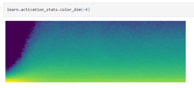
We see that the accuracy is quite poor, despite no symption of overfitting. Fastai learner has a
callback that allow us to see the mean, std and % of near zero activations. It is important to check the
stats on the last layers, as the early layers could show fairly low % of zero activations, but they
propagate relatively fast:

robust activations as they have more data points at the expense of lower gradient change frequency.

We can see that while it improve the performance of the model, the percentage of the near zero activations
remains high while its mean and sd are not as smooth as they should. We will try to adjust our learning
rate strategy, in the so called first cycle training. What we are going to do here is to change the learning rate,
starting with relatively low values first and increase them progressively, and at some point reduce it back
to low values. This will allow to train faster, avoid overfit and sharp local minimas, being located in the
smoother part of the loss. To help further, we will use momentum, particularly with low learning rates
where we will keep the direction of previous gradients.
def fit(epochs=1, lr=0.06):
learn = Learner(dls, simple_cnn(), loss_func=F.cross_entropy,
metrics=accuracy, cbs=ActivationStats(with_hist=True))
learn.fit_one_cycle(epochs, lr)
return learn


The model perform much better, but still one can see the % of zeros is very high. We can plot the histogram
of activations at each batch to see how there is quite some instability at the beginning, lossing time during
learning as activations collapsed several times.

Last but not least, we will try batch normalization to check if that leads to a smoother training process
over the batches and better performance. To motivate the need for batch normalization, note that
there is a permanent change in the distribution of the values from the previous outputs, due to
parameter/weight changes. If, for each layer and batch we normalize its means and sd, we can avoid
that to happen. That could lead to flattened activations,which is undesirable. To overcome that, we add two
learnable parameters gamma and beta, which allows for more flexibility in the amount of activation if that helps for learning.

This improve the performance of the model and shows a much better learning pattern across batches.
As claimed by the following paper, BatchNorm, we can use faster learning rate and still achieve better
and stable results.
Conclusions
We cover the main concepts behind convolutional neural networks aritmetic, and also show how they require
moderate batch sizes, differentiated learning rates and momentum, and batch normalization.
With all those tricks we are able to train stable and accurate computer vision models. In the next part
of this post, we will covert resnets, and essential architecture of modern computer vision networks.
The Link to the repo can be found here: REPO!
Comments
Post a Comment